8. The desktop app

GridSim.Wpf is the Windows control-room dashboard. It solves a network once per tick and shows the result as a live map, a column of system read-outs, and sixteen tabs that each read the same solved frame. It runs three kinds of feed through the same screens: a local live solve, a recorded run directory that you step through, and a stream from the GDA bridge. This chapter covers starting it, the window, the model picker, the map, the live view and its controls, the tabs, the asset explorer, run replay, bridge mode and settings.json. The browser version is summarised at the end.

The app is a WPF program (net10.0-windows), so it runs only on Windows. It builds on other systems.

Starting it

dotnet run --project src/GridSim.Wpf

Close the app before rebuilding: a running copy locks its own binaries (see ch. 1, Getting started). The window opens maximised, titled GridSim - GB Transmission Control - v<version> - <tier> licence, and starts solving at once.

Launch arguments

All arguments are optional. The app reads the raw command line (Environment.GetCommandLineArgs()), checks it (GridSim.Core.Presentation.DesktopLaunchArgs) and applies it.

• --zone <text> pre-selects the bridge ZONE picker: the first zone whose case name contains the text, ignoring case (--zone ukpn selects zone-ukpn).
• --back <days> pre-selects the bridge FROM picker. The value must be a whole number equal to one of the presets (9, 12, 14, 21, 30 or 60).
• --bridge-source <name> pre-selects the bridge SRC picker: presolved, estimated or live, ignoring case.
• --tab <text> opens on the first tab whose header contains the text, ignoring case, scanning left to right (--tab operator).
• One other word is the model text. The app opens on the first model-picker entry whose label contains it, ignoring case (case118, GB full, Replay). With no model text, it opens on the model you last used, and on the first entry in the picker if that model no longer exists.

Each flag takes its value as the next word, and that word is never the model text: --back 30 sets the look-back and leaves the model alone, and --tab OPERATOR on its own opens the last-used model on the OPERATOR tab.

The app refuses a command line it cannot honour. It shows a message listing every problem and closes with exit code 2 (a usage error, as in the CLI) instead of opening on something you did not ask for. It refuses:

• a value that matches nothing: a zone, tab or model text that no entry contains, a --back that is not a preset, or a source that is not one of the three;
• a --back that is not a whole number of days;
• a flag with no value after it, or followed straight by another flag;
• a flag given twice, or two model words (quote a label that contains spaces);
• an unknown option. Flags match exactly and case-sensitively, so --Zone is refused with a hint, and only the two-token form is read, so --zone=ukpn is refused with the right spelling.

The first three only pre-select pickers. They connect to nothing: the pickers act only once the Live bridge entry is selected (see Bridge mode). To boot into bridge mode, select Live bridge by model text and add the picker arguments:

dotnet run --project src/GridSim.Wpf -- bridge --zone ukpn --back 30 --bridge-source estimated

The window

The window has four horizontal bands.

Header (top). From left to right:

• NETWORK - the model picker. See The model picker.
• SOLVER - the power-flow engine, with a read-out beside it. See The solver picker.
• A find box. Type part of a substation name and press Enter: the map centres on the first bus whose name contains the text (ignoring case) and opens its fly-out. With no match the event log records No substation matching '...'.
• LOAD RUN... - opens a run directory for replay (Replaying a run directory).
• AUDIT LOG... - opens the audit-log window. Choose a gridsim-audit/1 log there with its own OPEN LOG... button. The optional anchor count and anchor head boxes (entry count and head hash recorded elsewhere) can be filled in first; a bad anchor shows NOT CHECKED: .... The whole hash chain is verified before anything shows, exactly as gridsim audit show does. A log that verifies lists every entry and the OK line; a log that does not verify shows only the TAMPERED verdict and no entries. See ch. 26, Audit log, deployment and assurance.
• On the right, the status lamp and the clock: the simulated clock, tick and the tick count.

Tab strip and tab content. Sixteen tabs (The tabs).

Transport bar. One playback bar under the tabs, visible from every tab (The transport bar).

Footer. A legend: ROUNDEL = SUBSTATION (ring colour = voltage) and LINE = CORRIDOR (dashes = power flow, colour = loading).

The status lamp

The lamp grades every solved frame in a fixed priority order, and shows the first condition that holds:

1. NOT CONVERGED - the power flow stopped without converging, so its voltages and flows are not an operating point. The lamp is red, and an alarm is raised.
2. FREQUENCY EVENT - the frequency is outside the operational band 0.2 Hz either side of the case's nominal (below 49.8 Hz or above 50.2 Hz on a 50 Hz case; exactly the edges are in band), or the RoCoF magnitude is above 1 Hz/s, the GB loss-of-mains relay setting (exactly 1 Hz/s is not an event). The web lamp applies the same rules.
3. VOLTAGE ALERT - the lowest bus voltage is below 0.94 pu or the highest is above 1.06 pu. Exactly 0.94 pu and 1.06 pu are in band.
4. CORRIDOR ALERT - a transmission boundary is over its limit.
5. SYSTEM NORMAL - none of the above.

A non-converged frame never shows SYSTEM NORMAL. A solver exception, or a frame the app cannot render, shows SOLVE FAULT with an alarm and an event-log line. On a bridge feed, a what-if state on the map prefixes the verdict with WHAT-IF, and a stream that has stopped shows STREAM LOST (Bridge mode).

The NETWORK tab

The NETWORK tab is the main screen and has three columns.

• Left: read-outs. SYSTEM FREQUENCY (a dial from 49.5 to 50.5 Hz, the value in Hz and the deviation from 50 Hz), DEMAND (GW), GENERATION (GW, labelled net bus injection: the sum of positive net bus injections, so generation at a bus with local demand is counted net of that demand), INERTIA (GVAs), LOSSES (MW), GRID SPEED (rpm) and TORQUE (MNm), the VOLTAGE BAND card (lowest to highest bus voltage, against the 0.94 - 1.06 band), and VOLTAGE BY LEVEL, one small gauge per nominal kV level showing its deviation from nominal.
• Centre: the map (The network map).
• Right: TRANSMISSION BOUNDARIES (each boundary with a loading bar, its percentage and its flow), ALARMS (up to 12 rows, newest first, with a CLEAR button), and the EVENT LOG (the newest 14 lines, newest first).

GRID SPEED is the frequency expressed as the speed of a two-pole machine: frequency / 50 Hz x 3000 rpm. TORQUE is the total generation divided by the angular frequency, P / (2 pi f), in MNm. Both follow the live frequency.

The model picker

The NETWORK picker lists every model the app can find, in this order. Labels are exactly as shown, except that when two entries would share a label (two gda-out/ or results/ folders with the same name under different parents) each gets its parent folder appended in brackets, so every label is unique.

Picker label	What it is	Where it comes from
GB reduced 10-zone	The reduced GB model. The default first entry.	data/uk next to the app
GB synthetic distribution depth	The GB model with synthetic distribution depth.	data/gb-synthetic
GB full 3539-bus transmission	The full GB transmission model.	data/gb-full
GDA <folder>	A model materialised by gridsim gda --out, one entry per sub-folder holding a system.json.	gda-out/
MATPOWER <case>	One entry per .m file, sorted by path.	data/matpower (recursive)
Replay <run>	A recorded run directory (Replaying a run directory).	results/ folders, or LOAD RUN...
Live bridge	A stream from the GDA bridge (Bridge mode).	Listed only when BridgeEndpoint is set

An entry appears only when its files are present. The three bundled GB entries and the MATPOWER entries come from the data/ folder that the build copies beside the executable. The app looks for gda-out/ and results/ in the application folder and in each of its seven parent folders, so they are found whether you run from the repository root or from bin/. A folder that cannot be read (access denied, a dropped network share) is skipped, and the event log names it. If no model is found at all, the app shows a message box and stays empty. Ch. 2, Loading networks describes the models themselves.

A model loads in this order: parse the case (MATPOWER cases are normalised for raw ohm and kW distribution files), give coordinate-less cases a tube-map layout, check the bus count against the licence, build the solver, load the map, start the first solve and fit the map. The licence gate counts buses only. The bundled GB and MATPOWER models are exempt. A GDA model above the active tier's bus limit is refused, with the reason on the event log (see ch. 4, Licensing and activation). A local model or replay that was running stays running after a refusal. A bridge feed is disconnected before the gate runs, so a refusal leaves it disconnected, and the refused entry stays selected in the picker.

Two behaviours depend on the model type:

• GB and GDA models run the day demand curve. The simulated clock starts at 08:00.
• MATPOWER cases have no demand profile. They hold their loads steady and re-solve the same operating point every tick, warm-started from the last converged solve.

A case that ships an authored asset-classes.json drives the live frequency through the asset-aware integrator, which is what makes the INVERTER FLEET tab live.

The solver picker

Choice	Engine
Auto	Chosen per network
Newton (dense)	Dense Newton-Raphson
Newton (sparse)	Sparse Newton-Raphson
Sweep (radial)	Backward/forward sweep

Auto picks the sweep for a strictly radial network, sparse Newton above 1,500 buses (LiveSolveSettings.SparseThresholdBuses), and dense Newton otherwise. The read-out beside the picker shows what runs: auto * Newton-Raphson (dense) under Auto, the engine name alone under an explicit choice, replay for a run directory and bridge for the bridge. Changing the solver rebuilds the running local model on the new engine and restarts its timeline. On a replay (pre-solved) and on the bridge (solved by the server) the picker is disabled, because the choice has nothing to rebuild. On the sparse engine the live view caps the solve at 40 iterations (LiveSolveSettings.SparseMaxIterations), does not enforce generator reactive limits, and skips the on-load tap-changer loop; the sweep also skips that loop. Engine behaviour is described in ch. 5, Running power flows.

The network map

The map draws substations as roundels and corridors as lines.

• Ring colour is the bus voltage, on every model. Blue is low, green is nominal, amber and red are high (see below).
• Line colour follows the colour mode (Colour modes). Dashes march along each line in the direction of the real-power flow. The animation takes at most one step per 65 ms (15.4 frames per second). Transformer branches are not drawn as animated corridors.
• Roundel size and ring weight follow voltage level. Models of up to 800 buses draw every bus at every zoom. Larger models draw the highest-voltage buses first and add lower-voltage ones as you zoom in. Hover and click hit only the buses being drawn.
• A minimap sits at the bottom left. Clicking inside it recentres the main view. It is not drawn when the view is too small: it needs a width and a height of at least 24 pixels and 24 pixels of spare height.
• The map title is GB TRANSMISSION NETWORK LIVE POWER FLOW, and a permanent hint line along the bottom edge lists the mouse actions and the map keys for the current feed: on a local model right-click trips, T trips the largest unit and . / , change the step; on a replay there are no trips; on a bridge right-click opens the what-if menu. Esc closes the detail fly-out.
• While a bridge query result is shown, a WHAT-IF banner across the top of the map carries the query title and its verdict (Bridge mode).

Moving around

• Scroll zooms about the cursor, by a factor of 1.15 per notch.
• Drag pans. A press that moves 3 pixels or fewer is a click.
• Fit (key F) fits the whole network to the view with a 36 pixel margin. The app also fits after every model load.
• Dive in (double-click). Double-clicking a substation centres it and zooms to six times the fit zoom. Double-clicking empty space zooms 1.6 times toward the cursor. The find box does the same dive-in for a named bus.
• Hover a bus for a tooltip: its name, its nominal kV, its solved voltage in pu and its demand in MW.
• Click a bus for a fly-out: the Voltage, Demand and Generation rows, and up to twelve connected branches with their loading. A branch fly-out shows its Type (Circuit or Transformer), Rating in MVA, Flow in MW (the larger of the two end flows) and Loading. OPEN IN EXPLORER selects the ASSETS tab and opens the bus or branch there. The close button on the fly-out, or Esc, clears the selection.

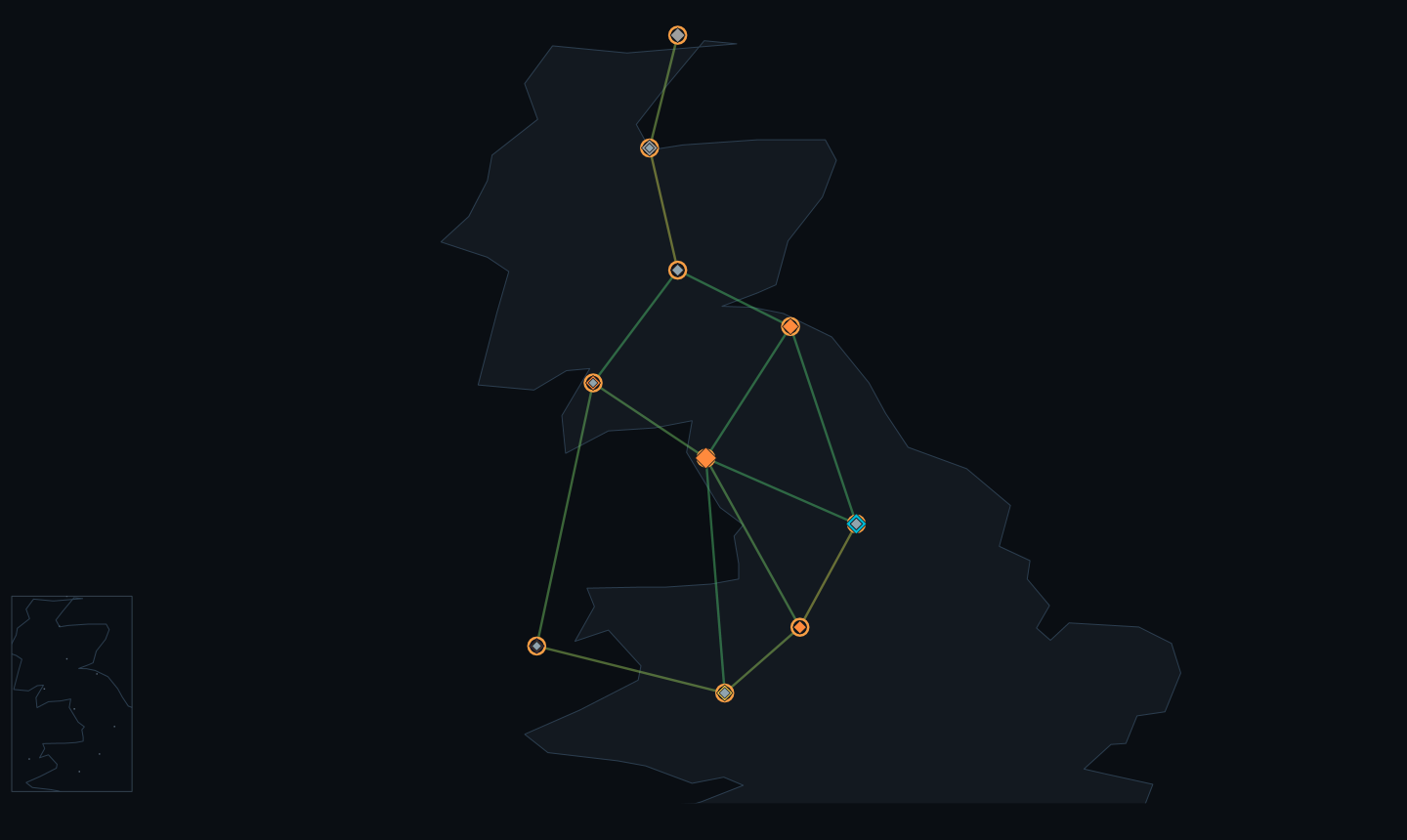
The screenshots in this chapter were captured on an earlier build. Their glyphs and some labels (a middle dot in the header clock, dashes in subtitles) differ from the current ASCII text, which the prose gives.

Colour modes

The colour button on the transport bar cycles LOADING, VOLTAGE, CONDITION and STRESS and back to LOADING. A legend panel at the bottom left of the map shows the ramp and its end labels for the current mode.

Mode	What colours the lines	Ramp	Legend ends
LOADING	Branch loading as a fraction of rating; a branch with no rating uses its flow against a 2,000 MW reference	Green at 0, amber at 0.6, red at 1.0 and above	0% to 100%
VOLTAGE	Mean voltage of the branch's two buses	Blue at 0.96 pu and below, green at 1.00, amber at 1.03, red at 1.06 and above	0.94 to 1.06
CONDITION	Mean condition index of the branch's two end buses (rings use the bus's own index)	Green healthy to red critical, amber at 0.5	healthy to critical
STRESS	Per-branch stress	Blue cool to red hot, amber at 0.5	cool to hot

Line colours step in 12 bands. Transformer branches are excluded from the line colour bands. CONDITION and STRESS are fed only by the bridge stream. On any other feed, or before the first bridge overlay arrives, lines draw the lowest colour. CONDITION recolours the rings by condition index as well as the lines, but only once an overlay has arrived: until then the rings stay voltage-coloured, as they do in every other mode.

The FLEET button overlays the generation fleet on the map: one diamond per unit, coloured by fuel and sized by capacity. The map toggles M (minimap), C (coastline), B (boundary cuts) and G (GSP areas) are listed under Keyboard shortcuts. The DNO, GSP and ASSETS buttons overlay real geography: DNO licence-area boundaries, GSP regions, and geocoded REPD/DUKES assets coloured by technology. They are dimmed and disabled unless that geography has been materialised locally under gda-out/geo (files dno_areas.geojson, gsp_regions.geojson and assets.geojson). The three buttons and the D, R and A keys are enabled together when any one of the three files loads, not per file; a file that cannot be read leaves its layer empty and the event log says Geography layer not loaded: <file>: <reason>. The app reads gda-out/geo next to the executable, or, when run from a repository clone, in a parent folder up to the repository root (the folder holding GridSim.slnx), never above it. Imported test cases have none.

The live view

A local model solves once per timer tick on a background thread. The timer interval is 800 ms divided by the playback speed. A solve never overlaps the previous one: if the previous solve is still running when the timer fires, that tick is skipped.

Controls

• PAUSE / RESUME stops and restarts the timer. While paused the map animation also stops.
• STEP sets the simulated time advanced by each solve: 1 ms, 10 ms, 100 ms, 1 s, 10 s, 1 min, 5 min or 20 min (default 20 min). The frequency model integrates the swing equation at the step size. Fine steps let you watch RoCoF and the nadir after a trip in slow motion; coarse steps sweep the demand curve.
• x1 cycles the playback speed x1, x5, x15, x60. It sets how often a solve is attempted: every 800, 160, 53.3 or 13.3 ms. It does not change the STEP size. The real rate is lower when a solve takes longer than the interval.
• The colour, FLEET, DNO, GSP and ASSETS buttons act on the map.

Frequency display

The frequency comes from a swing-equation integrator advanced at the STEP size, with a small ambient load imbalance (0.08 % of base demand) that keeps the dial moving, at the case's own nominal frequency. The dial sweeps 120 degrees either side of centre at a deviation of 0.5 Hz, and its end labels follow the nominal. The dial's track is drawn over the same 240 degrees, so each labelled end is full scale, and its green band covers the 0.1 Hz green zone of the number. The GRID SPEED dial on the GENERATION tab uses the same geometry. The number is green below 0.1 Hz deviation from nominal, amber from there to the edge of the operational band, and red outside it, by the lamp's own rule, so at exactly 49.8 Hz or 50.2 Hz on a 50 Hz case both the number (amber) and the lamp read in band. When a case carries no usable inertia data the integrator uses a substitute fleet inertia: a value under 100 MW.s is replaced by 4 s on the fleet's MVA base (LiveSolveSettings.MinInertiaMwS and FallbackInertiaH).

Right-click: trip

Right-clicking a bus on a live model trips its largest infeed: the unit generating the most at that bus now, by live output (power-flow-only devices, the slack balancer and voltage-control units, are never chosen). The loss enters the frequency integrator and plays out at the current STEP. The event log records the unit, its MW, the RoCoF and the nadir, an alarm is raised, and the GENERATION & INERTIA tab computes its trip comparison. The header lamp is left to the next frame's lamp rule, so a small trip that keeps the frequency in band does not light FREQUENCY EVENT. Pressing T trips the largest online unit on the whole system. A bus with no generating unit logs No generation to trip at <name>, and T with no generating unit logs No generation to trip.

A trip is a frequency what-if: the unit's output enters the integrator as a loss, but the unit stays in the dispatch, so it is still the largest infeed on the next frame. A second trip of the same unit in the same run is therefore refused, with the reason in the event log, rather than counted again. Loading a model starts a new run.

On a replay or a bridge feed the app has no local solver. In replay, a right-click on a bus logs TRIP is not available on this feed (replay or bridge stream). In bridge mode a right-click opens the bridge menu (Bridge mode).

The tabs

There are sixteen tabs, in this fixed order. All read the one solved frame; none re-solves the base case. The EXPERIMENTAL tab does its work only while it is the selected tab; switching to it computes the current frame at once. A tab that is also a chapter 10 view is marked, and that chapter explains how to read it.

Tab	What it shows
NETWORK	The map, the system read-outs, the boundaries, alarms and event log, described above.
GENERATION & INERTIA	Fuel mix split into synchronous and converter-connected plant, live system inertia, and the TSGB device what-if.
THE MACHINE	The grid as one rotating mass: FUEL IN, the shaft (power by voltage level), the instruments (speed, commanded and delivered torque, TORQUE GAP), MAINS CLOCK DIVERGENCE, the grid battery and regeneration, POWER OUT, and the electrical instruments (voltage, reactive balance, tap positions).
SCADA	A telemetry-style points list with navigation to the asset explorer. See ch. 10, Analysis views.
OPERATOR	The generation stack, boundary transfers and the dispatch view. See ch. 10.
MARKET	Wholesale and balancing prices: imbalance price, market index, BSUoS, constraint cost, carbon, demand and interconnector flows. The price fields fill only from a bridge stream; on other feeds only demand, renewable share and an indicative carbon intensity (computed from the dispatch) are live. See ch. 10.
NESO RP1	The stability panel: purchased time, inertia split, credible-loss and correlated-trip risk. See ch. 10.
MECHANICAL	The per-machine plant view: stored kinetic energy per unit, P-Q capability and RoCoF relay margins. See ch. 10.
HUMAN SCALE	The same quantities in everyday units. Presentation only.
SPEED DOMAINS	The distributed-inertia view: coherent speed domains and dominance. Experimental.
INVERTER FLEET	Authored per-asset dynamics: fleet net response, per-class online MW and state of charge, trips and the Loss-of-Mains deficit. It shows OFF unless the case ships asset-classes.json.
EXPERIMENTAL	The physical-law conformance audit with its hard-gate verdict, and the provenance-tagged experimental models (reciprocity, continuum wave, flow tracing, carbon intensity). Flow tracing and carbon intensity are skipped on models above 1,500 buses (trace skipped (>1500 buses), carbon shows -). The continuum-wave model reads "needs per-machine inertia" and is not built when the solve did not converge, when there are no generators, or when any generator has no inertia constant.
HARMONICS	A reference panel for gridsim harmonics: what the study covers, the command line, and the schema names. It runs no study. See ch. 17, Harmonic studies.
CYCLE	The resident analysis cycle's budget read-out: high-tier jobs met or missed, utilisation and per-job outcomes. See ch. 10.
ASSETS	The asset explorer (The asset explorer). See ch. 10.
ABOUT	The release number, build, runtime and active licence, and where a crash log is written.

An unhandled exception on the UI thread or on any other thread writes a crash log, shows a message box naming its path and ends the app. A failed background task that nobody awaited writes a crash log only, with no message box, and the app keeps running.

The transport bar

One bar sits under the tabs and its contents change with the feed.

Control	Live	Replay	Bridge
PAUSE / RESUME / PLAY	yes	yes (label PLAY when stopped)	opens playing (label PAUSE); PAUSE holds the display
restart, previous, next, scrubber, frame read-out	hidden	shown	hidden
STEP	shown	hidden	hidden
x1 speed	yes	yes	disabled (the server paces the stream)
SOLVER	yes	disabled (pre-solved)	disabled (solved by the server)
Colour, FLEET, DNO, GSP, ASSETS	yes	yes	yes
ZONE, FROM, SRC	hidden	hidden	shown

The asset explorer

The ASSETS tab is a navigable stack of pages over every asset class in the running model. The landing page has one card per class with a live count and a headline metric:

Card	Opens	Headline metric
GENERATORS	The generating fleet by fuel	Dispatched output in GW
GENERATOR PHASORS	Every generator's voltage-current phasor	Voltage-angle spread across the network, in degrees
INTERCONNECTORS	The GB import links, with signed flow	Net flow in GW, labelled NET IMPORT or NET EXPORT, or BALANCED below the shared 0.5 MW idle cut-off (the GENERATION tab's)
TRANSFORMERS	GSP and grid transformers by voltage band	Mean loading of rated transformers
CABLES & LINES	Transmission corridors, ordered by stress	Peak circuit loading
SUBSTATIONS	Every bus	Count of buses outside 0.94 - 1.06 pu
TAP CHANGERS	On-load tap changers and the buses they regulate	Count held within their deadband, shown as n / N

Each fleet page lists its items; click an item for its detail page. Detail pages cross-link: a circuit to its two substations, a substation to its plant and circuits, a generator back to its bus. The BACK button pops one page, ASSETS returns to the landing page, and the breadcrumb shows the trail. The header strip shows the simulated time and tick of the displayed frame. The visible page refreshes with every frame while the ASSETS tab is selected, and not while another tab is showing.

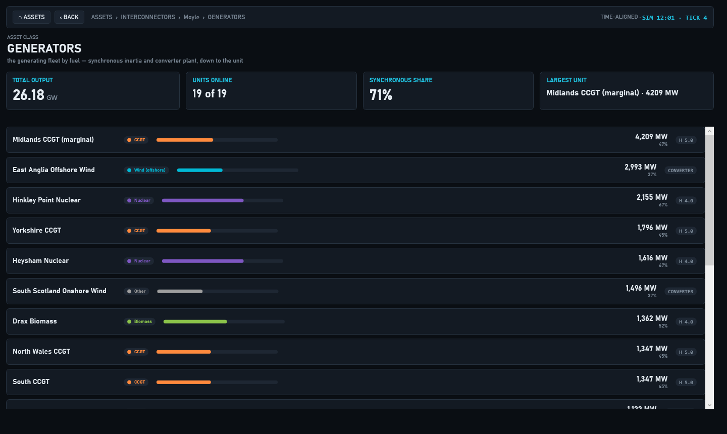
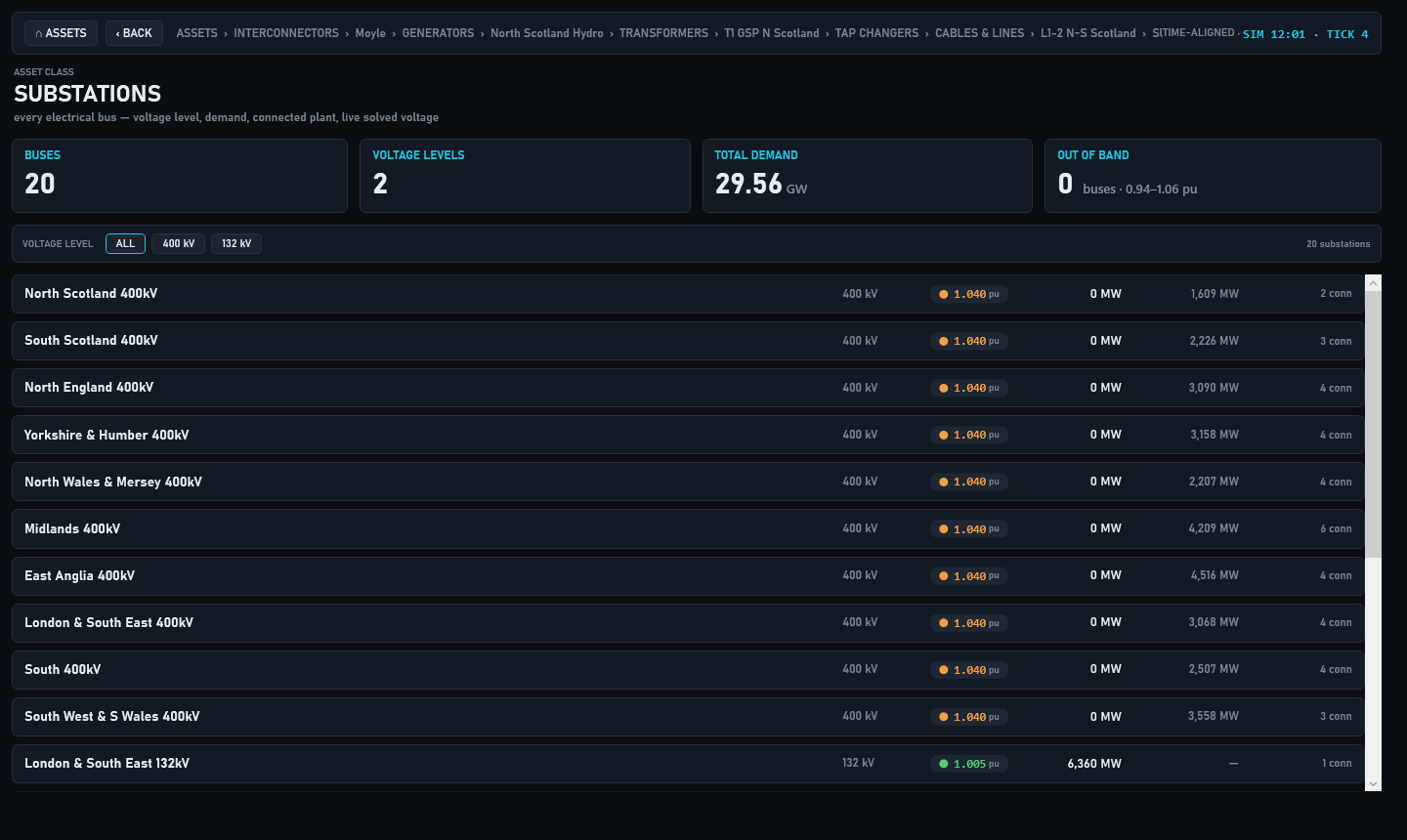
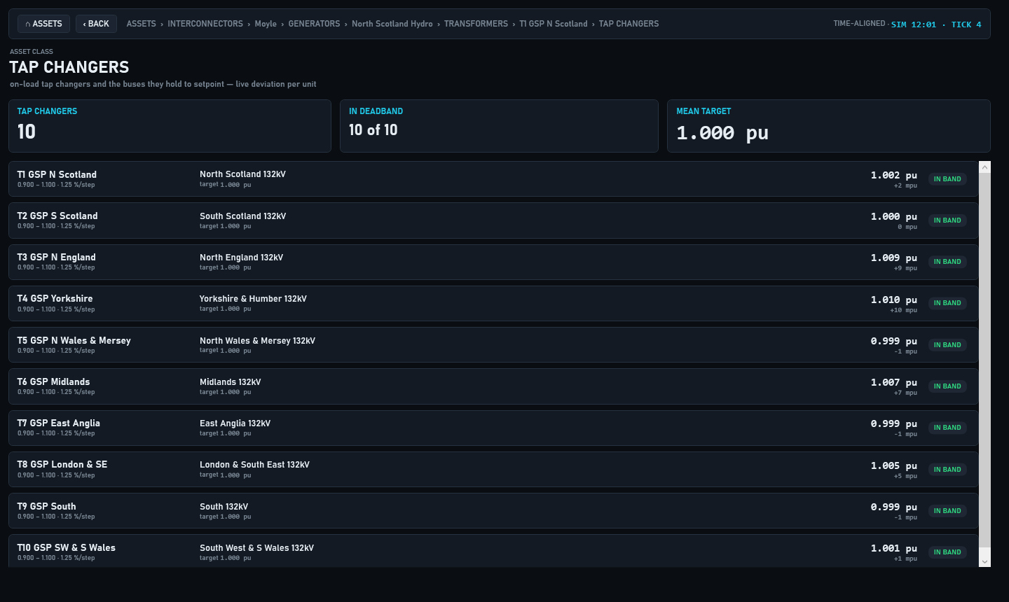
Several routes lead into the explorer: OPEN IN EXPLORER on the map fly-out, a click on a SCADA point, and the cards on the landing page. The first two select the ASSETS tab by its name. In bridge mode, a substation page opened from the map also asks the bridge for that bus's per-asset data at the stream's historical instant (generator envelope, battery storage, tap-changer wear and consumers). The page says when none resolved or why the query failed.

Replaying a run directory

The app can step through a recorded run instead of solving live. A run directory is the output of gridsim transient or gridsim gda-replay; see ch. 5, Running power flows and ch. 31, Exports and formats.

What is discovered

A directory is a run when it has an exports/ folder holding JSON files named slice-<n>.json or state-<n>.json, where <n> is an integer. The app lists, as Replay <folder name>, every sub-folder of every results/ folder in the application folder and its seven parent folders that is a run. LOAD RUN... opens a folder browser for a run anywhere else, adds it to the picker and selects it; a run already listed (the same folder) is selected, not added again. A folder that is not a run is refused with the event-log line Not a run directory (no exports/slice-*.json or state-*.json).

Playing a run

A replay opens paused on frame 0, with the solver read-out replay. Frames play in the numeric order of the file names. The event log records the frame count, the number of buses, and for a run of more than one frame the first and last frame labels. The transport bar shows:

• PLAY / PAUSE - frames advance at the timer interval (800 ms divided by the speed), and playback stops on the last frame. PLAY on the last frame restarts from frame 0.
• restart - back to frame 0.
• previous / next - step one frame. This is the frame stepping control.
• the scrubber - a slider across every frame, snapping to whole frames. Dragging to frame 0 restarts the timeline exactly like restart does.
• the read-out - frame 12/480 * <label>, with the frame number from 1.

Each frame carries its own solved voltages and flows. A sidecar CSV beside the exports is matched to frames on its tick or index column. A transient run writes timeseries.csv, which supplies frequency, RoCoF, generation, demand, the clock and the frame label. A gda-replay run writes state-estimate.csv, which has no frequency, RoCoF, generation or demand columns, so it supplies only the clock (from time_utc) and the frame label. For every value a sidecar does not supply, including all four scalars on a gda-replay run, generation and demand are summed from the frame, the frequency is the model's nominal frequency and RoCoF is 0. Frames from an exported transient run are a sample of its slices, so the replay steps through snapshots, not every slice. A time-integrated read-out, such as THE MACHINE's accumulators, restarts on every restart, on every step back and on every backward scrub (including a scrub to frame 0), so it never double-counts a replay.

Bridge mode

Selecting Live bridge in the picker streams topology and solved states from a GDA bridge server. There is no local solver and no local model files, and the server paces the stream (2 frames per second). The entry exists only when BridgeEndpoint in settings.json is set. A fresh install leaves it blank, so a new install lists no bridge. Starting and configuring the server is ch. 24, The GDA bridge. Using the estimated-state source is ch. 23, Replaying estimated states.

Three pickers appear on the transport bar. Changing any of them restarts the stream on the same connection.

• ZONE - the network to stream. The choices are NGED - Midlands/SW/S.Wales (zone-nged, the default), UKPN - London/South East/East (zone-ukpn), SSEN - N.Scotland/Southern (zone-ssen), SPEN - Scotland/Merseyside (zone-spen), NPg - North East/Yorkshire (zone-npg), ENWL - North West (zone-enwl), GB full (gb-full) and GB spine - GSP-level (gb-spine).
• FROM - the historical instant the stream starts from: 9 days ago (the default), 12 days ago, 2 weeks ago, 3 weeks ago, 30 days ago or 60 days ago. Every preset is behind the 169 hour no-forward-inference horizon, so the server never rejects it. With no preset selected the look-back is 9 days.
• SRC - the reconstruction that plays. PRESOLVED is the demand-scaled re-solve lake. ESTIMATED is the measurement-fitted lake, where each frame carries a chi-square quality block shown on the status pill; the pill turns red when the fit fails its quality test. The pill adds WARNING: robust re-weighting (IRLS) hit its cap, weights not settled when the server sends irlsCapReached and a robust fit's re-weighting stopped on its cap; no current server sends that field, so the warning does not appear today. LIVE is a static network with only the system scalars moving.

The server paces the stream, and the bar opens playing (the button reads PAUSE). PAUSE holds the display on the frame showing: the map, its overlays and dash animation, the HUD and the OPERATOR and MARKET tabs stop changing, and the pill reads PAUSED * <zone> * display held, stream still running. The stream itself keeps running on the server, and the app keeps only the newest frame. PLAY shows that newest frame and follows the stream again. Changing ZONE, FROM or SRC, or RETURN TO LIVE, also resumes playing.

Status pill and HUD. A pill at the top left of the map shows the connection state: CONNECTING, LIVE * streaming <zone>, ESTIMATED * <zone> * <quality>, RESTARTING, QUERY, WHAT-IF, HORIZON REJECTION * stream stopped, BRIDGE FAULT * disconnected, or a connect or restart failure with its reason. WHAT-IF shows only while a what-if state is on the map; after a scalars-only or failed query the pill returns to LIVE with the next frame, and a failed query also raises an alarm. When the stream stops (a fault or a horizon rejection) nothing on screen is live any more: the header lamp reads STREAM LOST, an alarm says the map shows the last frame received, the HUD is hidden, the OPERATOR, MARKET and NESO RP1 bridge blocks are cleared, and a right-click on the map offers Reconnect to the bridge. Changes of ZONE, FROM or SRC in quick succession restart the stream one at a time, and a burst of changes ends on the newest selection. A HUD at the bottom right shows INERTIA in GVA.s, FRAGILITY (a condition index with a trend cue) and RoCoF HEADROOM in Hz/s. FRAGILITY is coloured on the stream's 0 to 100 fragility scale. The streamed network carries no machine inertia constants, so the dashboard's INERTIA tile shows the stream's own inertia figure (or - when the stream sends none) rather than a model total of 0. The OPERATOR and MARKET tabs fill from the stream's operator and market blocks, and CONDITION and STRESS colouring works.

Right-click. A right-click opens a menu of queries that the server evaluates at the stream's historical instant:

• on a bus, Feasibility: +500 MW here (<bus>) and Scenario: trip the largest generator at <bus> (the largest physical unit generating there, by the same rule as a local trip), or, when no unit generates at that bus, Scenario: trip the largest unit in the model (none generating at <bus>);
• on a branch, Scenario: trip this (<branch>);
• while a result is shown, Return to live stream.

The server picks the element to trip by name (technical chapter 9), so a trip is not sent for an element with no name or whose name also matches another element in the model: the branch item is shown disabled with the reason, and a generator trip logs it.

A result that carries a converged solved state goes through the same path as a live frame: the map, the header lamp (marked WHAT-IF), the read-outs and the tabs all show the what-if state, and live frames are held off. A solved state that did not converge is never drawn: the WHAT-IF card shows the verdict with a red badge and says the solve did not converge. The right-hand column shows a WHAT-IF card with the verdict, the binding constraint and the violations, and a RETURN TO LIVE button.

settings.json

%LOCALAPPDATA%\GridSim\settings.json holds the state the app restores. The app writes it when the window closes. A missing file means the defaults apply. An unreadable or malformed file also leaves the defaults in force, but the event log says why, and the app does not overwrite that file when it closes, so a hand edit (such as BridgeEndpoint) with a typo is kept for you to fix. A write that fails does not stop the window closing.

Key	Default	Meaning
LastSource	none	Label of the model selected when you last closed the app. Used only when LastSourcePath is absent or matches nothing.
LastSourcePath	none	Full path (or bridge URL) of the model selected when you last closed the app. Labels can repeat; the path cannot, so this is matched first.
ColorVoltage	false	true restores VOLTAGE colouring, false LOADING. CONDITION and STRESS are saved as LOADING.
Fleet	false	The FLEET overlay.
Minimap	true	The minimap.
Coast	false	The coastline.
Boundaries	false	The boundary cuts.
GspAreas	false	The GSP areas.
DnoAreas	false	The DNO overlay.
GspRegions	false	The GSP region overlay.
Assets	false	The geocoded assets overlay.
BridgeEndpoint	empty	WebSocket URL of the GDA bridge. Non-empty adds the Live bridge entry.

The licence is resolved separately, offline: the GRIDSIM_LICENCE environment variable, then %LOCALAPPDATA%\GridSim\licence.gridsim, then the free Personal tier. See ch. 3, Configuration and ch. 4, Licensing and activation.

Keyboard shortcuts

The shortcuts are window-wide and act on the map. They are ignored when keyboard focus is in a text box, a password box or a combo box, and for Ctrl and Alt chords, so typing a substation name never trips a unit. Click the map to return keyboard focus to it.

Key	Action
F	Fit the network to the view.
M	Toggle the minimap.
C	Toggle the coastline.
B	Toggle the boundary cuts.
G	Toggle the GSP areas.
D	Toggle the DNO overlay. Needs local geography.
R	Toggle the GSP regions. Needs local geography.
A	Toggle the geocoded assets. Needs local geography.
T	Trip the largest online unit on the system (live feed only).
.	A finer STEP.
,	A coarser STEP.
Esc	Clear the selection.

Performance

The fixed numbers are these: the map animation takes at most one step per 65 ms; the timer interval is 800 ms divided by the speed; solves never overlap; models above 1,500 buses solve on the sparse engine under Auto; and models above 800 buses draw only their higher-voltage buses until you zoom in. Solve timings by engine are in ch. 28, Benchmarking and GPU. The CYCLE tab reports the measured base-solve time of the model on the machine in front of you.

The web app

GridSim.Web is a browser version of the same control room, built on the same GridSim.Core solve. It runs on any platform. It differs from the desktop app in these ways:

• It has no ZONE, FROM or SRC pickers. A bridge session is chosen by its address.
• It adds the tabs TRIP / DEVICE and CONFORMANCE, and AUDIT LOG is a tab, not a button. It has no ABOUT tab on its full strip.
• Its HARMONICS tab runs the study in the page, where the desktop tab is a reference panel.
• A raw public-data replay session shows a reduced tab strip.

Limits

• CONDITION and STRESS colouring have data only on a bridge feed.
• DNO, GSP and ASSETS geography needs gda-out/geo materialised locally; no geography ships with the app.
• The Live bridge entry is absent until BridgeEndpoint is set by hand.

See also

• ch. 1, Getting started - building and the rebuild file-lock
• ch. 2, Loading networks - what the model picker finds
• ch. 5, Running power flows - the engines and the run directories the app replays
• ch. 10, Analysis views - the analysis tabs one by one
• ch. 14, Frequency studies - tripping an infeed and watching the dial
• ch. 23, Replaying estimated states and ch. 24, The GDA bridge - the bridge in depth
• ch. 19, CLI reference - the verbs that produce the data the app shows